Part 1
- 假設我們的數學模型如下:
y = axp+bxq 而資料點如下:x 1 2 3 4 5 6 7 8 9 10 y 2 14 43 90 160 255 378 530 715 930 試用下述兩種方法求出參數 a、b、p、q 的最佳值,並算出最小平方誤差總和。
- 將 a、b、p、q 全視為非線性參數,以 fminsearch 來求出最佳參數值。
- 將 a、b 視為線性參數,使用「左除」來計算之;並將 p、q 視為非線性參數,使用 fminsearch 來求出其最佳值。
- 在進行最小平方法時,為何要取平方誤差而不是直接取絕對值誤差?
Ans:因為我們可以藉由對總平方誤差的微分而得到一組線性方程式,進而得到一組解析解。若是採用絕對值誤差,則微分後並無法得到線性方程式,因此不容易求解。 - 對一指數函數 $y=ae^{bx}$ 求最小的擬合誤差,下列何者不可直接使用?
- 變形法 + 最小平方法
- 混成法
- 最小平方法
- Simplex 下坡式搜尋
- 變形法的目的是將一個非線性的數學模型,轉換成只包含線性參數的數學模型,以方便進行資料擬合。請問進行轉換後,目標模型的一般形式為何?請使用一個方程式來表示。
Ans: $f(X, y)= \alpha_1*g_1(X, y) + \alpha_2*g_2(X, y) + \cdots + \alpha_n*g_n(X, y)$,其中 $n$ 是可變參數的個數,必須等於原模型的可變參數個數。 - 請從 MATLAB 讀入太陽黑子資料 sunspot.dat(位於 {matlab root}\toolbox\matlab\demos\ 之下),並請用你覺得最適合的方式,來尋找數學模型,並畫出曲線擬合結果。
Part 2
- Difference between interpolaton and data fitting: What is the key difference between interpolation and data fitting?
- Polynomial order for prediction: Please explain briefly how come the increase in the polynomial order for polynomial fitting does not always lead to a better prediction.
- Quadratic form:
Express the following equation in quadratic form $\mathbf{x}^TA\mathbf{x}$, where $\mathbf{x}=[x, y, z]$ and $A$ is symmetric:
$$x^2+2y^2+3z^2+4xy+6yz+8xz$$
Solution: $$ x^2+2y^2+3z^2+4xy+6yz+8xz = \left[\begin{matrix} x\\ y\\ z\\ \end{matrix}\right]^T \left[\begin{matrix} 1 & 2 & 4\\ 2 & 2 & 3\\ 4 & 3 & 3\\ \end{matrix}\right] \left[\begin{matrix} x\\ y\\ z\\ \end{matrix}\right] $$ - Gradients:
Give the simplest matrix format of the following expressions
- $\nabla \mathbf{c}^T\mathbf{x}$
- $\nabla \mathbf{x}^T\mathbf{x}$
- $\nabla \mathbf{c}^TA\mathbf{x}$
- $\nabla \mathbf{x}^TA\mathbf{c}$
- $\nabla \mathbf{x}^TA\mathbf{x}$ (where $A$ is symmetric)
- $\nabla \mathbf{x}^TA\mathbf{x}$ (where $A$ is asymmetric)
- $\nabla (\mathbf{x}^TA\mathbf{x}+\mathbf{b}^T\mathbf{x}+\mathbf{c})$ (where $A$ is symmetric)
Solution:- $\nabla \mathbf{c}^T\mathbf{x} = \mathbf{c}$
- $\nabla \mathbf{x}^T\mathbf{x} = 2\mathbf{x}$
- $\nabla \mathbf{c}^TA\mathbf{x} = A^T\mathbf{c}$
- $\nabla \mathbf{x}^TA\mathbf{c} = A \mathbf{c}$
- $\nabla \mathbf{x}^TA\mathbf{x} = 2A\mathbf{x}$ (where $A$ is symmetric)
- $\nabla \mathbf{x}^TA\mathbf{x} = (A+A^T)\mathbf{x}$
- $\nabla (\mathbf{x}^TA\mathbf{x}+\mathbf{b}^T\mathbf{x}+\mathbf{c}) = 2A\mathbf{x}+\mathbf{b}$ (where $A$ is symmetric)
- Derivation of LSE: Use matrix notations to prove that the least-squares estimate to $A\mathbf{\theta}=\mathbf{b}$ is $\hat{\mathbf{\theta}} = (A^TA)^{-1}A^T\mathbf{b}$.
- Derivation of weighted LSE: Sometimes we want to assign different weights to different input/output pairs for data fitting. Under this condition, the objective function for solving $A\mathbf{x}=\mathbf{b}$ can be expressed as $e(\mathbf{x})=(A\mathbf{x}-\mathbf{b})^TW(A\mathbf{x}-\mathbf{b})$, where $W$ is a diagonal matrix of weights. Please derive the weighted least-squares estimate to $A\mathbf{x}=\mathbf{b}$ based on the given objective function.
- Find a point that has the minimum total squared distance to 3 lines:
Given 3 lines on a plane:
$$
\left\{
\begin{matrix}
x & = & 0\\
y & = & 0\\
4x+3y & = & 12\\
\end{matrix}
\right.
$$
You need to find a point P that has the minimum total squared distance to these 3 lines. You can formulate this problem into a least-squares problem by noting the formula of the distance between a point and a line. In particular, the total squared distance can be formulate as $E(\theta) = ||A\theta-\mathbf{b}||^2$ where $A$ and $\mathbf{b}$ are known, while $\theta$ is unknown (the point to be found), and the solution can be obtain from MATLAB by left division.
- Give the value of $A$ and $\mathbf{b}$ for solving this problem.
- When P is found, what is the distance to each side of the triangle (formed by the 3 lines)?
Hint: This can be solved by Cauchy-Schartz inequality.
- Distance of a point to a hyperplane:
- Given a point $P=[x_0, y_0]$ in a 2D plane, what is the shortest distance between P and a hyperplane $L: ax+by+c=0$?
- Given a point $P=[x_0, y_0, z_0]$ in a 3D space, what is the shortest distance between P and a hyperplane $L: ax+by+cz+d=0$?
- Given a point $P=[x_1, x_2, ..., x_d]$ in a d-dim space, prove that the shortest distance between P and a hyperplane $L: a_0+\sum_{i=1}^d a_i x_i=0$ is given by $$ \frac{|a_0+\sum_{i=1}^d a_i x_i|}{\sqrt{\sum_{i=1}^d a_i^2}} $$
- Find a point that has the minimum total squared distance to a set of lines or planes:
This problem is an extension to the previous one. In other words, the problem can be formulated as a least-squares problem where the point P can be found by $\mathbf{b}$ left divided by $A$.
- You need to find a point P that has the minimum total squared distance to a set of $n$ lines: $$ \left\{ \begin{matrix} a_1x+b_1y+c_1=0\\ a_2x+b_2y+c_2=0\\ ...\\ a_nx+b_ny+c_n=0\\ \end{matrix} \right. $$ Then what are the formulas for $A$ and $\mathbf{b}$?
- You need to find a point P that has the minimum total squared distance to a set of $n$ planes: $$ \left\{ \begin{matrix} a_1x+b_1y+c_1z+d_1=0\\ a_2x+b_2y+c_2z+d_2=0\\ ...\\ a_nx+b_ny+c_nz+d_n=0\\ \end{matrix} \right. $$ Then what are the formulas for $A$ and $\mathbf{b}$?
- Function for line fitting via LSE:
Write a function lineFitViaLse.m to perform line fitting via least-squares estimate ("left division" or "right division" in MATLAB), with the following usage:
theta = lineFitViaLse(X), where X is a 2-by-n dataset matrix, with each column being an observation. In other words, for a column in X, the second element is the output while the first element is the input part of the observation. You function should return a column vector $\theta=\left[\begin{matrix}a\\b\end{matrix}\right]$, where the fitting line can be expressed as $y=ax+b$.Test case: planeFitViaLse(X) returns [0.5323; 10.1155] when
X=[38 93 34 68 33 3 58 87 11 22;25.5 61.2 31.5 43.8 29.5 7.9 38.2 57.6 18.4 25.5].
If you plot the line, the result will be like this: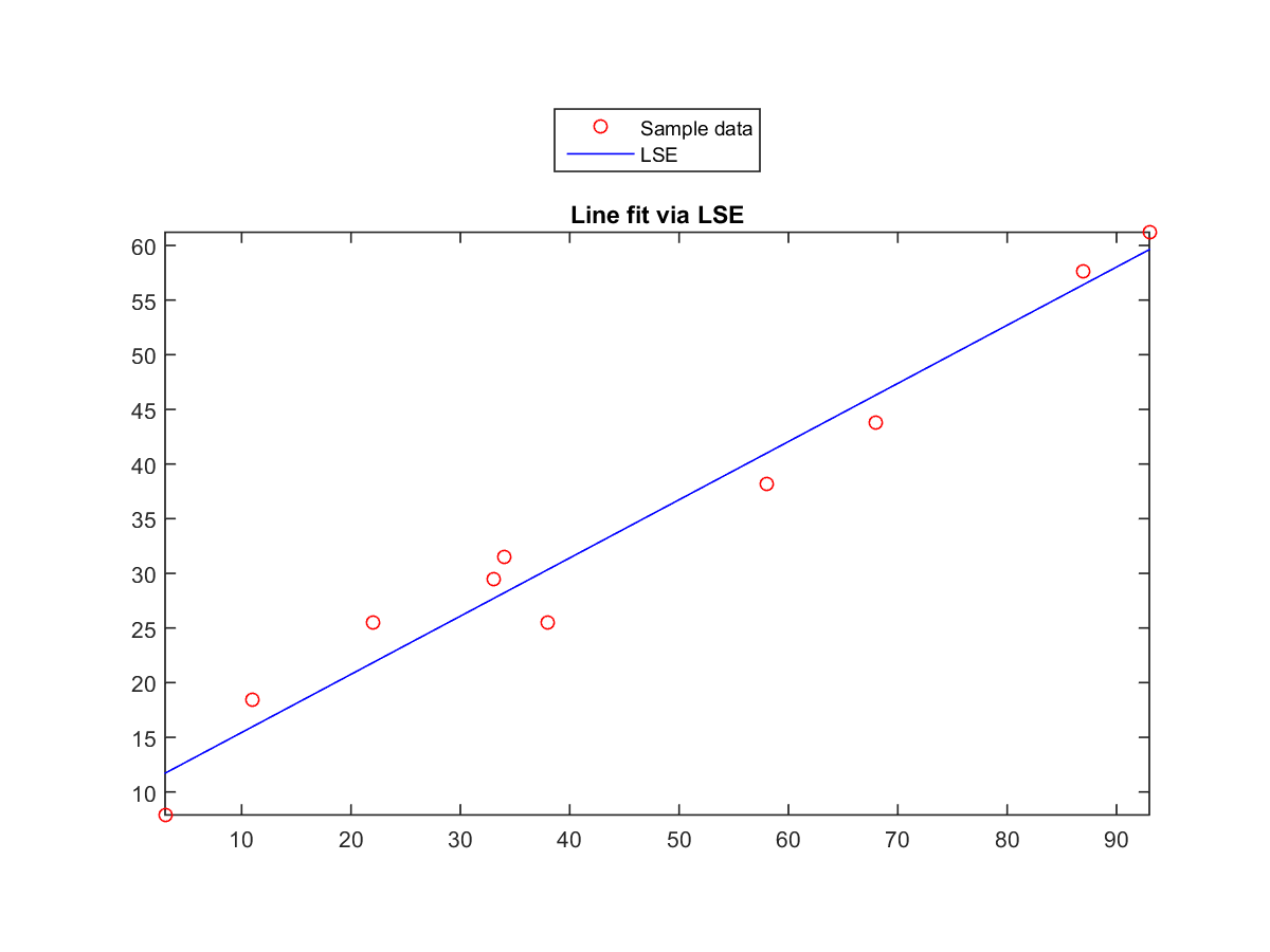
- Function for plane fitting via LSE:
Write a function planeFitViaLse.m to perform plane fitting via least-squares estimate ("left division" or "right division" in MATLAB), with the following usage:
theta = planeFitViaLse(X), where X is a 3-by-n dataset matrix, with each column being an observation. In other words, for a column in X, the last element is the output while all the other elements are the input part of the observation. You function should return a column vector $\theta=\left[\begin{matrix}a\\b\\c\end{matrix}\right]$, where the fitting plane can be expressed as $y=ax_1+bx_2+c$.Test case: planeFitViaLse(X) returns [2; 1; 3] when
X=[38 93 34 68 33 3 58 87 11 22;69 43 42 92 60 57 6 82 1 83;148 232 113 231 129 66 125 259 26 130].
- Function for min. total squared distance to a set of planes:
Write a function minSquaredDist2planes(P) to return a point in a 3D space that has the shortest total squared distance to a set of m planes defined by a 4-by-m matrix P, where the $i$th column represents a plane of p(1,i)*x+p(2,i)*y+p(3,i)*z+p(4,i)=0.
Test cases:
- minSquaredDist2planes([1 6 5 2 1;1 7 7 1 0;1 1 9 1 7;0 7 1 -5 -7]) returns [4.3136; -4.5380; 0.5579].
Here is a test script which can be run with minSquaredDist2planes.p:
- Transform nonlinear models into linear ones:
Transform the following nonlinear models into linear ones. Be sure to express the original nonlinear parameters in terms of the linear parameters after transformation.
- $y=\frac{ax}{x^2+b^2}$
- $(x-a)^2+(y-b)^2=c^2$
- $\frac{x^2}{a^2}+\frac{y^2}{b^2}=1$
- $y=ae^{\left(-\frac{x-c}{b}\right)^2}$
- All the nonlinear models that can be converted into a linear ones (as listed in the text or slides).
- Hybrid method for data fitting: Please describe how to use the hybrid method for data fitting of the model $y=ae^{bx}+ce^{dx}$, and explain the method's advantages.
- Hybrid method after transformation for data fitting:
The equation for a general ellipse model can be expressed as follows:
$$
\left(\frac{x-c}{a}\right)^2+\left(\frac{y-d}{b}\right)^2=1
$$
where a, b, c, and d are 4 parameters of the model.
- In order to use separable least squares for curve fitting, we need to transform the original model into the one with as many linear parameters as possible. Please transform the above model, and specify the linear and nonlinear parameters after transformation.
- Please describe how you approach the curve fitting problem after the transformation.
- Order selection for polynomial fitting based on leave-one-out cross validation:
In this exercise, you need to write a MATLAB function that can select the order of a fitting polynomial based on LOOCV (leave-one-out cross validation) described in the class. More specifically, you need to write a function polyFitOrderSelect.m with the following input/output format:
[bestOrder, vRmse, tRmse]=polyFitOrderSelect(data, maxOrder) where- "data" is the single-input-single-output dataset for the problem. The first row is the input data, while the second row is the corresponding output data.
- "maxOrder" is the maximum order to be tried by the function. Note that maxOrder should not be greater than size(data,2)-1. (Why?)
- "bestOrder" is the order that generates the minimum validation RMSE (root mean squared error).
- "vRmse" is the vector of validation RMSE. (The length of vRmse is maxOrder+1.)
- "tRmse" is the vector of training RMSE. (The length of tRmse is maxOrder+1.)
- Note that to alleviate the problem of truncation and round-off error, you need to perform z-normalization on the input part of the dataset. More specifically, to follow the spirit of LOOCV, you need to find $\mu$ and $\sigma$ based on the training set only, and then use them to normalize both the training and validation sets.
- If you don't do z-normalization, sometimes you get the right answers, sometimes you don't. This is simply because the data is generated randomly in our judge system. That is, z normalization is likely to give you a more reliable answer to polynomial fitting.
- For a specific polynomial order, LOOCV needs to use one entry as the validation set and all the others as the training set for each iteration. The final RMSE is defined as the square root of SSE (sum of squared error) divided by data count. As a result, for a complete loop of LOOCV, the data counts for validation SSE and training SSE are $n$ and $n(n-1)$, respectively, where $n$ is the size of the whole dataset. (Check out the following code template, where dataCount is $n$.)
- Here is a code template:
Here is a test example:
- Origin-centered ellipse fitting:
In this exercise, we will transform a nonlinear ellipse model (centered at the origin) into a linear one, and use it for data fitting.
- The equation for a ellipse centered at the origin can be expressed as follows: $$ \left(\frac{x}{a}\right)^2+\left(\frac{y}{b}\right)^2=1 $$ Apparently there are 2 nonlinear parameters a and b in the above equation. Please transform the above equation into a model with linear parameters. In particular, you need to express the original parameters in terms of the linear parameters.
- We have a sample dataset of 100 points which are located near a ellipse (centered at the origin) in a 2D plane. The data can be plotted as follows:
If your linear model is the same as mine, you should be able to plot the model as well as the dataset, as shown next: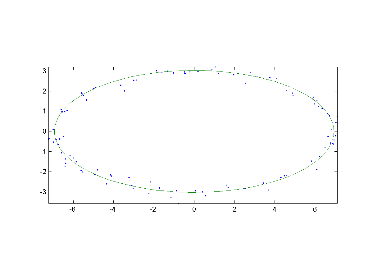
- Circle fitting:
A circle can be described as
$$(x-a)^2+(y-b)^2=r^2,$$
where $(a, b)$ is the center and $r$ is the radius of the circle. We can transform the circle model into a linear one by noting that:
$$
\left[ 2x, 2y, 1\right]
\left[ \begin{matrix}a\\b\\r^2-a^2-b^2\end{matrix} \right]
=x^2+y^2
$$
Write a function circleFit.m with the following usage:
output = circleFit(X, method) where- X: an 2-by-n dataset matrix, with each column being an observation.
- method: 1 for using the above transformation method, 2 for using the transformation method plus "fminsearch".
- output: a column vector of the derived $[a, b, r]^T$.
Here are two test examples which can be run with circleFit.p:
- Ball fitting:
A ball can be described as
$$(x-a)^2+(y-b)^2+(z-c)^2=r^2,$$
where $(a, b, c)$ is the center and $r$ is the radius of the ball. We can transform the ball model into a linear one by noting that:
$$
\left[ 2x, 2y, 2z, 1\right]
\left[ \begin{matrix}a\\b\\c\\r^2-a^2-b^2-c^2\end{matrix} \right]
=x^2+y^2+z^2
$$
Write a function ballFit.m with the following usage:
output = ballFit(X, method) where- X: an 3-by-n dataset matrix, with each column being an observation.
- method: 1 for using the above transformation method, 2 for using the transformation method plus "fminsearch".
- output: a column vector of the derived $[a, b, c, r]^T$.
- Ellipse fitting:
In this exercise, you need to view a nonlinear ellipse model into a model with both linear and nonlinear parameters. And then we shall empoly LSE (least-squares estimate) for linear parameters and fminsearch for nonlinear parameters. The equation for a general ellipse model can be expressed as follows:
$$
\left(\frac{x-c_x}{r_x}\right)^2+\left(\frac{y-c_y}{r_y}\right)^2=1,
$$
where the parameter set is $\{c_x, c_y, r_x, r_y\}$. In particular, it is rather easy to reorganize the model and treat $\{c_x, c_y\}$ as nonlinear parameters, while $\{r_x, r_y\}$ can be identified via LSE which minimize the following SSE (sum of squared error):
$$
sse(data; c_x, c_y, r_x, r_y)=\sum_{i=1}^n \left[\left(\frac{x_i-c_x}{r_x}\right)^2+\left(\frac{y_i-c_y}{r_y}\right)^2-1\right]^2,
$$
where $data=\{(x_i, y_i)|i=1\cdots n\}$ is the sample dataset.
Write a function ellipseFit.m with the following I/O formats to perform ellipse fitting:
[theta, sse]=ellipseFit(data); where- Inputs:
- data: the sample dataset packed as a matrix of size $2 \times n$, with column $i$ being $(x_i, y_i)^T$
- Outputs:
- theta: $\{c_x, c_y, r_x, r_y\}$, which is the identified parameter sets, with the first two identified by fminsearch (with the default optimization options) and the second two by LSE (on the transformed linear model). Note that when using fminsearch, the initial guess of the center should be the average of the dataset.
- sse: SSE (sum of squared error)
[sse, radius]=sseOfEllipseFit(center, data); where- Inputs:
- center: $[c_x, c_y]$
- data: the sample dataset packed as a matrix of size $2 \times n$, with row $i$ being $(x_i, y_i)^T$
- Outputs:
- sse: SSE
- radius: $[r_x, r_y]$, which is identified by LSE.
Here is a code template:
We have a sample dataset of 100 points which are located near a ellipse in a 2D plane. Here is a test example for ellipse fitting:
- Inputs:
- Ellipse fitting via coordinate optimization:
Repeat the previous exercise using coordinate optimization. In other words, the parameters of the ellipse model can be divided into two disjoint sets. For each of the set, you can derive a linear model with respect to the set.
- Guess good values of $[r_x, r_y]$ and use the linear model of $[c_x, c_y]$ to obtain $[c_x, c_y]$. What is the linear model? What is the SSE (sum of squared error) in terms of the original model?
- Guess good values of $[r_x, r_y]$ and use the linear model of $[c_x, c_y]$ to obtain $[c_x, c_y]$. What is the linear model? What is the SSE in terms of the original model?
- Can you use coordinate optimization to find $[c_x, c_y, r_x, r_y]$? Why or why not? Please write a script to verify your answer.
MATLAB程式設計:進階篇